The 7th order polynomial in the "Fitting Noise" example in the Polynomial Equations pitfall was a perfect example of this phenomena. When you add more parameters, a small change in one parameter can have a chain reaction effect on the other parameters. This can cause wild shifting of the parameter values that can cause the curve fitting to converge on a local minimum, or even diverge.

This is much more serious when dealing with equations containing nested or rational terms because you increase the chance of creating a statistical dependence among two or more parameters. When this occurs, the confidence intervals for these parameters are inflated dramatically.

Additionally, a large number of curve fitting iterations also shows that the equation has redundant parameters, because the algorithm found a very narrow valley in the SS space. This valley has a slope that has a very slight curvature, so the algorithm is using a small step size, causing it to “slow down”. As a result, the curve fit will take a long time to converge, if it does at all.

The best way to determine if such a problem exists is to inspect the confidence intervals of each parameter in the equation you are fitting.

Here are the ANOVA tables from the "Fitting Noise" example. Notice that the confidence intervals for the quadratic equation are very small:



Compare that with the 7th order polynomial. Notice that the confidence intervals (and Standard Error) are very wide. The P-values for all of the parameters are all greater than .20, indicating that none of them are statistically significant to the model. In other words, they're not accurately describing the relationship between the equation and the data. However, notice that the r-squared value is higher.

A customer called up one day with a real problem. He was attempting to fit a theoretical model for an optics experiment. When he fitted the equation he noticed that the curve wasn't following the trend as well as he felt it could, and the parameter values from the curve fit didn't correspond to his estimates.

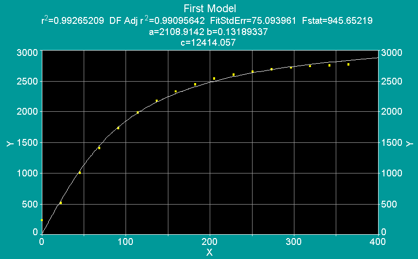
This was the equation and resulting curve fit:




Judging from the graph, he had a good point about the line not fitting the first data point and the last three data points very well. No matter how much he modified the values for the parameters, nothing changed.

In this case, there were two problems:
1) The K*B terms were acting like a constant
2) When parameter C is increased in value, the 1 in the denominator is rendered insignificant by the fitting, which causes large shifts in parameter B. In effect, this made the three parameter model a two parameter model.

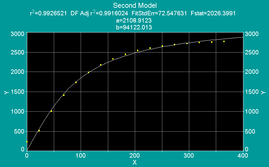
This doesn’t mean that the equation is invalid, but all we can do is to eliminate the statistical ratio between parameters C and B. Because they are inversely correlated, the best way to fix the problem is to eliminate one of the parameters. For this case, B was removed from the equation. This is the resulting equation and curve fit:





But wait - the graphs look identical! How can this be?

A comparison of the ANOVA tables shows what happened:



Notice that the confidence limits for B and C are very wide in the first model. This is also reflected in the P-value. In the second model, the r-square is the same as the previous fit, but the F-Statistic is much better. In addition, the confidence intervals for the parameters are much more respectable.

Parameters B and C in the first model were in fact inversely correlated. Notice that if you divide C by B, you end up with the virtually the same value as the B parameter in the second model. (C/B) = 94121.91537755, compared with B = 9412.01297. Although the two curve fits are visually the same, the second curve fit is much better from a statistical perspective.

This is why inspecting the confidence intervals for the parameters is very important.

Now this brings up the question - how do you simplify a model? Well, there are a variety of strategies that you can use. Some tricks you can use include the following:

1) Removing one or more parameters
2) Scaling the equation; you cancel out a large number by dividing it by that same number elsewhere in the equation
3) Use a less complex model
4) Change the model to use a logarithmic scale; try using log(y) = ( ... ) instead of y =( ... )

Here's a simple example of how to do this. This is an equation that shows statistical dependence between parameters A, C and D:




If you expand the equation, the statistical dependence is very clear:




Since "AD" and "(A/C)" are essentially constants, we simply replace them with a single variable, which restores the statistical independence of the parameters. The added bonus? You can now use a linear least squares procedure!