Sample polynomial equation:

Pros:
Able to fit a wide variety of data sets
Numerically easy to fit, as it uses linear least squares procedures

Cons:
Extrapolation can be very risky
Tendency to fit noise, especially with higher order equations
Unable to fit straight lines

How to identify problem:
Graphical inspection

Generally speaking, polynomial equations actually do a very good job of fitting a variety of data set profiles. One major problem lies in the area of extrapolation. This is the process of using your curve fit model to predict data values beyond the X data range provided for the curve fit.

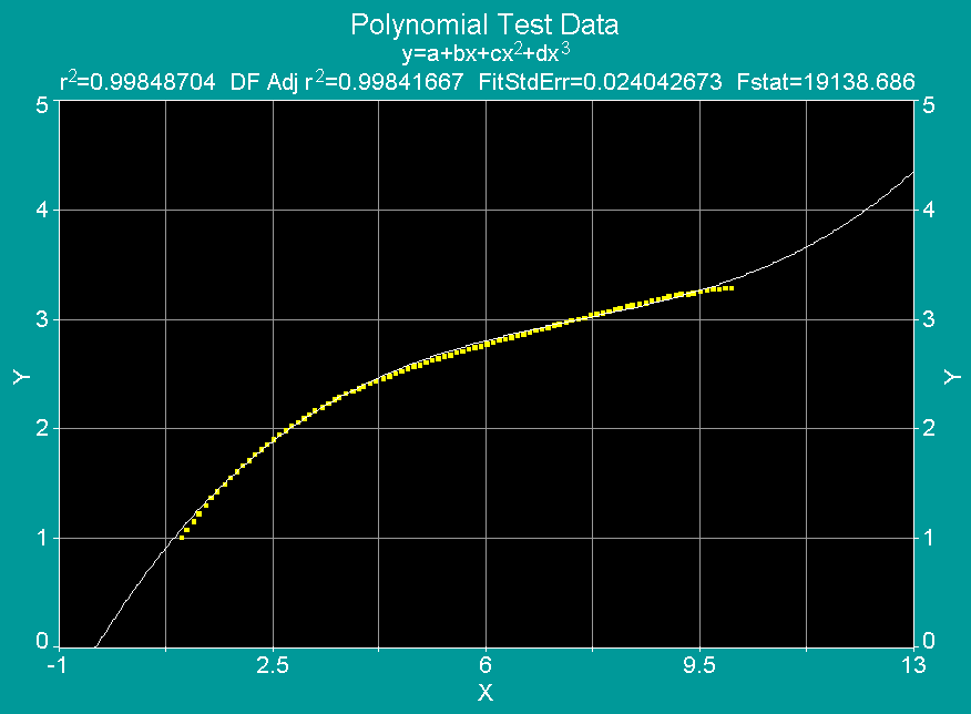
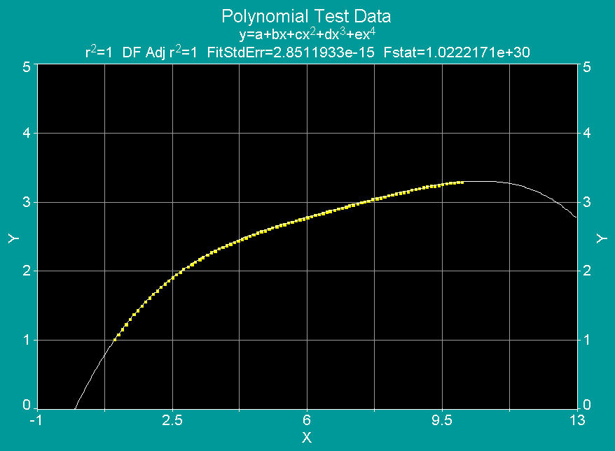
The main problem with using polynomials for extrapolation lies in the fact they have a strong tendency to change direction once they leave the X data range. Here are two examples of this below:

Example 1: Fitted curve fit goes up abruptly



Example 2: Fitted curve fit levels off slightly, and then goes down



If you wish to perform extrapolation, it's strongly recommended to inspect the area of interest before doing so. In both of these examples, performing any extrapolation, because neither curve fit really follows the data set profile outside of the X data range.

You could fix the extrapolation problem by using a different model, but the better solution is to obtain data for the X range you were originally trying to extrapolate to, and then perform the curve fit again.

The worst characteristic of polynomial equations is their tendency to fit noise within a data set. If your data doesn't have much noise or outliers, then they can generally be used safely. Otherwise, you will obtain a very strange curve fit.

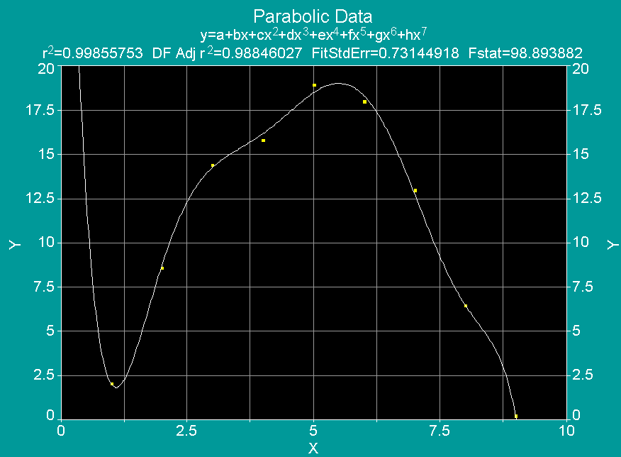
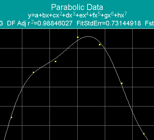
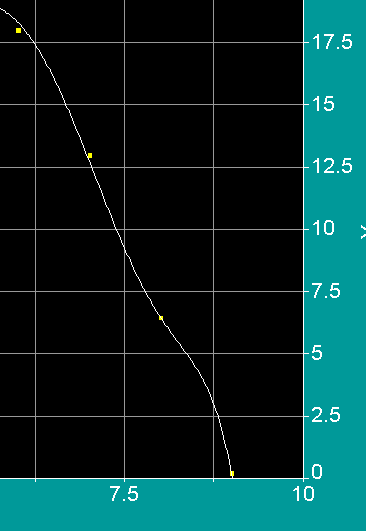
In this example, we were attempting to fit a 7th order polynomial equation to a slightly noisy data set has a quadratic equation profile. Notice that the resulting curve fit isn’t following the data trend at all because the noise is being fitted instead. You are essentially ending up with a “connect the dots” curve fit.




So you might think - what's the problem? Well, there are three major problems with this model. We will focus on three sections of the graph:


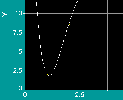
Problem #1: Extrapolation around the first data point

Notice that the curve fit comes down from infinity, goes through the first data point, overshoots it, and then travels back up. This behavior makes any extrapolation before or even near the first data point unreliable.




Problem #2: Fitting noise in the middle of the data set

The data points in the middle could be fitted much better. The peak is shifted over too far to the right, which would also make interpolation unreliable. This is being cause by the small amount of noise.




Problem #3: Strange behavior at end of data set

The last three data points are basically forming a straight line. Notice that the curve fit “squiggles” out before reaching the last data point.




There's another bonus pitfall in this curve fit. Did you notice it?
Hint: Look at the information at the top of the graph, and it doesn't deal with numbers.


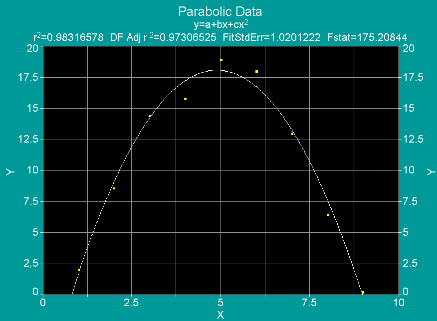
Here's a much better curve fit, which uses a quadratic equation:


This is a much better curve fit. Notice that the r-square is lower than the previous fit, but there are two things to notice:

1) The curve fit clearly follows the data trend, which will give more realistic values when performing interpolation and/or extrapolation.

2) Only a minimal amount of noise is being fitted.

The bonus pitfall - the previous curve fit used eight parameters for only nine data points! By contrast, this model only used three and resulted in a better fit. This will be elaborated in the section Redundant Parameters.

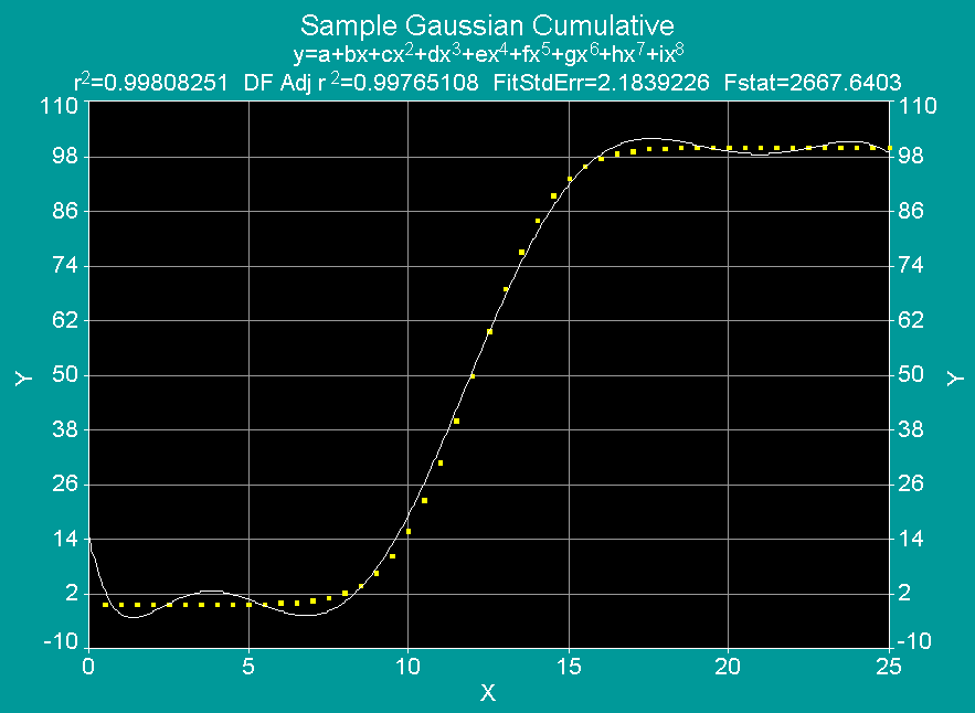
Polynomial equations are not a good choice when you are attempting to fit a data set that had a profile that combines curves and straight lines. When a polynomial is fitted to a straight line, it will become unstable and you will get a "Sine wave" effect.

This is an example, using a 10th order polynomial to curve fit a data set, which is in what's called a "Sigmoid" profile.

Notice how this 10th order polynomial fits the middle portion of the data set, but becomes unstable at the ends of the X data range, where it's a straight line. Polynomial equations will create their characteristic “sine wave” pattern when they are fitted to straight lines.