| Linear and Non-Linear Least Squares Procedures:
How They Are Different |
|
Linear vs. Non-Linear Equations
The objective of all curve fitting is
to find the best combination of parameter values in a given equation or model
that will minimize the residual sum of squares. This is the sum of the squared
distance between the Y data value and it’s predicted Y value. This is also
called the Chi-Square. Depending on the relationship of the parameters with respect
to each other, you will need to use either a linear or non-linear algorithm.
A linear equation is one whose
parameters appear linearly in the expression. The famous quadratic equation
from trigonometry is an example equation that is linear in all three parameters:
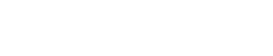
Linear equations only refer to
the relationship between the parameters and the terms in the equation, not
to the graphical appearance of the equation.
Linear equations are solved in
a single step using a linear Least Squares matrix procedure, by taking the partial
derivatives with respect to each parameter.
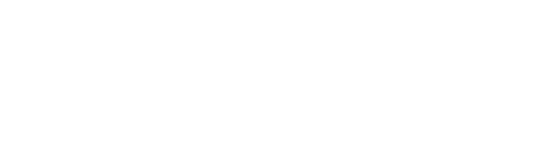
Non-linear equations, on the other
hand, require an iterative curve fitting procedure because the partial derivatives
for each parameter would include one or more of the other parameters. Often,
these equations include nested terms, like the Gaussian Peak equation (amplitude
version) you see here, that’s linear with parameters a and b, but non-linear
with parameters c and d.
Linear Least Squares Procedure
The linear least squares procedure is rather straight forward, and is discussed
in any book in linear algebra.
Using a linear LS procedure, linear equations are solved very quickly. The partial
derivatives with respect to each parameter is calculated. This is an example
with the quadratic equation above:
This is the Chi-Square function we are trying to minimize: 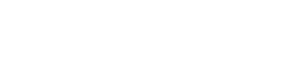
To minimize the function, we take the partial derivarive with respect to each
parameter, and set each equal to zero. Mathematically, this will break down
to a series of three simultaneous equations:
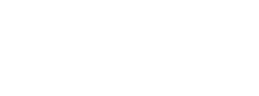
Now we are left with nothing more than a few summations and a solution of three
simultaneous equations. The final solution will provide the values of the parameters
a, b, and c that will minimize the Chi-Square function.
This is considerably faster computationally that the procedures required for
non-linear equations.
Non-Linear Least Squares Procedure
A non-linear least squares procedure is more complicated, and requires a few extra
steps:
1) Specify the equation that
you want to fit to the data
You have to provide an equation. Contrary to many people's beliefs, the algorithm
won't find the best fitting equation for you.
2) Provide
an initial set of estimates for the parameters in the equation
All non-linear curve fitting algorithms require a starting point. You only need
to be "in the ballpark" as they say. You can get these values from
basic estimation, "trial and error" or experience. It doesn't need
to be exact, unless you have a very complex equation. Either way, the better
the estimate, and better the curve fit. (This will be discussed in more detail
in Local Minimum Traps)
3) Specify convergence criteria and constraints
Most algorithms will automatically converge at 1e-8, but you can change this.
Some parameters may require a constraint for the model to be valid, like "B
must be greater than 0", "C must be between 1 and 2.5", etc.
In the Gaussian Peak example, parameter D must not be equal to 0.
4) Continue iterating
until the curve fitting algorithm converges
The algorithm will begin the computations. Some of the most popular non-linear
fitting algorithms are Newton’s Method, Method of Steepest Descent, Simplex,
or Levenburg-Marquardt. The algorithm will modify each parameter value until
the algorithm converges an a final solution based on the convergence criteria,
or fails to converge.
Issues
With Non-Linear Least Squares Procedures
There are three issues with non-linear least squares procedures that must be taken
into consideration:
1) It can be very time consuming
for large data sets
Although current implementations of non-linear algorithms are fast, they must
calculate a point by point sum of squares for each iteration. If you have a
very large data set, say 20,000+ data points, the curve fit may take a long
time to converge. For example, Levenburg-Marquardt requires a matrix inversion
and computation of the partial derivatives for each iteration.
2) The minimum sum of squares
isn't guaranteed, unlike the linear least squares procedure.
Unlike linear least squares algorithms, non-linear algorithms don’t guarantee
that the minimum sum of squares will be found. Sometimes, you may find a local
minimum instead of the true global minimum, where the sum of squares is minimized.
(This is covered a little later in Local Minimum Traps)
3) You are unable to obtain an exact solution
To calculate an exact least squares solution, you would minimize the sum of
squares to the full floating point precision of the machine. For an Intel 486/Pentium
series processor, this is 19 digits. A non-linear fit reaches the exact solution
asymptotically because the tolerance of convergence is always less than the
floating point precision of the computer. Potentially, you can see large differences
between a linear and non-linear curve fit using the same data set and equation.